


Analysis Overview
To understand why vibration analysis is useful and what it entails, we must first think of a simple mass spring damper model shown in Figure 14.

Figure 14: A simple single-degree-of-freedom system is represented where m is the mass, k is the spring constant, c is the damping coefficient, x represents the displacement from equilibrium and f defines the force acting on the mass as a function of time.
As review, some simple equations which describe the motion of this system and define key parameters are listed in Table 1. For those that are unfamiliar, there are plenty of resources out there that can provide more information on free vibration of single degree of freedom systems.
| Equation | Description |
|---|---|
 |
Differential equation of motion |
 |
Natural frequency as radians per second |
 |
Natural frequency as hertz |
 |
Damping ratio |
 |
Quality factor |
To understand why a vibration test engineer cares about these parameters, let’s take a look at a transmissibility plot shown in Figure 15. Transmissibility looks at how a SDOF system responds to a base excitation with a given damping and natural frequency. When the excitation frequency is much larger than the system’s natural frequency, the system isolates that base vibration. When the system’s natural frequency is much larger than the base excitation frequency the system will neither amplify nor dampen an input vibration. The worst case scenario is when the input frequency is equal to the system’s natural frequency which will amplify that input by a factor approximately equal to Q.

Figure 15: The transmissibility illustrates how a SDOF system will respond to a base excitation. This plot was taken from Tom Irvine’s vibrationdata publications that have some supporting information.
Most systems in the real world can’t be represented by a SDOF system; but every structure, no matter how complex, can be factored down to individual single-degree-of-freedom (SDOF) systems. And most real world excitations are not perfect sine waves but rather a collection of sine waves. Nevertheless, vibration analysis is used to predict how a system will react to a given input and provides the tools for an engineer to ensure survivability of his/her system. But all this is only made possible when the vibration environment is understood and known, which is why we do vibration testing!
Simple Analysis in the Time Domain
When analyzing vibration data in the time domain (amplitude plotted against time) we’re limited to a few parameters in quantifying the strength of a vibration profile: amplitude, peak-to-peak value, and RMS. A simple sine wave is shown in Figure 16 with these parameters identified.

Figure 16: A simple 60 Hz sine wave is shown with the amplitude, peak-to-peak, RMS, frequency, and period identified.
- The peak or amplitude is valuable for shock events but it doesn’t take into account the time duration and thus the energy in the event.
- The same is true for peak-to-peak with the added benefit of providing the maximum excursion of the wave, useful when looking at displacement information, specifically clearances.
- The RMS (root mean square) value is generally the most useful because it is directly related to the energy content of the vibration profile and thus the destructive capability of the vibration. RMS also takes into account the time history of the wave form.
Vibration is an oscillating motion about equilibrium so most vibration analysis looks to determine the rate of that oscillation, or the frequency which is proportional to the system’s stiffness. The number of times a complete motion cycle occurs during a period of one second is the vibration’s frequency and is measured in hertz (Hz). For simple sine waves the vibration frequency could be determined from looking at the waveform in the time domain; but as we add different frequency components and noise, we need to perform spectrum analysis to get a clearer picture of the vibration frequency.
Any waveform is actually just the sum of a series of simple sinusoids of different frequencies, amplitudes, and phases. A Fourier series is that summation of sine waves; and we use Fourier analysis or spectrum analysis to deconstruct a signal into its individual sine wave components. The result is acceleration/vibration amplitude as a function of frequency, which lets us perform analysis in the frequency domain (or spectrum) to gain a deeper understanding of our vibration profile. Most vibration analysis will typically be done in the frequency domain.
To illustrate how an FFT can be used, let’s build a simple waveform with three different frequency components: 22 Hz, 60 Hz, and 100 Hz. These frequencies will have amplitude of 1g, 2g, and 1.5g respectively. The following figure shows how this waveform looks a little confusing in the time domain and also illustrates how the signal length affects the frequency resolution of the FFT.

Figure 17: Constructed waveform with 22, 60, and 100 Hz frequency components is shown at varying sample lengths and with noise to illustrate usefulness of FFT analysis.
If we sample this wave at a 500 Hz rate (500 samples per second) and take an FFT of the first 50 samples we’re left with a pretty jagged FFT due to our bin width being 10 Hz (Fs of 500 divided by N of 50). The amplitudes of these frequency components are also a bit low. But if the range is extended to the first 250 samples as shown then the FFT is able to accurately calculate both the frequency and amplitude of the individual sine wave components.
Not that the “pure” waveform didn’t look confusing enough in the time domain; but if broadband noise is added as shown in the bottom plots then the waveform becomes even less distinguishable. This is the power of an FFT; it is able to clearly identify the major frequencies that exist to help the analyzer determine the cause of any vibration signal.
Fourier transforms perform an integral from negative infinity to positive infinity; but one can only acquire data over a discrete time period. So a Fourier transform must repeat the signal infinitely to perform the transform. When the acquired data begins and ends at 0, or if there are an integer number of cycles, then this infinite repetition will cause no problems. But if these are not true, there will be leakage in the frequency domain because the signal is distorted as shown in Figure 18.

Figure 18: The time-window effects are shown when using a FFT analyzer without windowing (or rather a uniform window) are shown. (A) represents an integer number of cycles so that the spectrum has a clear spectral line. (B) and (C) represent time signals where there are a half integer number of periods, but with different phase relationships, which gives a different discontinuity and spectral leakage.
Remember that a Fourier transform looks to calculate a series of sine waves to represent the data. If there is a discontinuity in the data (by not beginning and ending at 0 or not having an integer number of cycles) then the FFT analyzer will need many terms to approximate the apparently discontinuous signal.
In order to minimize this error, windows are used to better make the signal appear periodic for the FFT process. The most common windows are the rectangular window, the Hanning window, the flattop, and the force/exponential window (used for impact testing). The important thing to understand is that all windows distort the data. They are a necessary evil sometimes; but aren’t always required if the vibration tester can satisfy Fourier’s request by completely observing the signal in one sample of data. For more information check out Midé’s blog on Fourier transform leakage. When looking at software packages, an option for windowing is important for many applications.
In real world applications there will typically be many different frequency components of a vibration profile as well as mechanical and electrical noise. Let’s look at some data taken on a passenger car engine while it was idling and do some vibration analysis. This data was generated with a Slam Stick vibration data logger as part of a how-to video series if you're interested in some more details about the test setup.

Figure 19: A car’s engine during idle clearly shows the 30 Hz dominate frequency which equals twice the crank shaft rotation frequency of 15 Hz (900 RPM) where a peak is also visible.
We can use spectrum analysis of the vibration profile to indicate what the engine’s crank shaft rotation speed was. This is a 4-cylinder 4-cycle engine. The engine operates with two pairs of pistons moving out of phase with each other and two piston combustions per crank shaft rotation; so the dominant frequency of the engine’s vibration will be twice the crank shaft rotation speed (here’s a nice video on how a 4-stroke engine works). In the FFT there is clearly a dominate frequency at 30 Hz or 1,800 RPM which tells us that at idle the crank shaft is rotating at 900 RPM (or 15 Hz) where there is also a peak in the FFT. The use of an FFT in our vibration analysis gave clues on what was causing the measured vibration.
In many applications the vibration frequency will change with time and you can run into trouble if you only look at the FFT. Let's zoom out of the area where the car engine is running at a relatively fixed rate, and compute an FFT of the entire signal. In this test the engine sat off for a period of time, idled, then the engine was revved before letting it idle again and finally turning it off. The vibration frequency changed pretty dramatically throughout the test; but the FFT doesn't capture that. We know from the previous plot that when it was idling there was a fairly significant dominant vibration frequency of 30 Hz; but this peak gets muted when you try and look at the FFT of a changing vibration environment.

Figure 20: The time history and FFT are shown from a Slam Stick mounted to an engine block while it was revved to change the dominate frequencies.
In this example, and others where the vibration frequency changes with time, we need a spectrogram. A spectrogram works by breaking the time domain data into a series of chunks and taking the FFT of these time periods. These series of FFTs are then overlapped on one another to visualize how both the amplitude and frequency of the vibration signal changes with time. Turn this three dimensional surface plot of FFTs on its side, add a color scale to represent the amplitude (often works best when you look at the color/amplitude on a logarithmic scale) and you're left with a spectrogram!
Back to that car engine example where the engine was revved for a bit. The spectrogram shown below illustrates how the dominate frequencies change with time in relation to when the car engine was idled and revved. Using a spectrogram the analyzer gains a much deeper understanding of the vibration profile and how it changes with time.

Figure 21: Spectrogram of car engine shows how crank shaft speed change (when engine is revved) affects vibration frequencies which become apparent in spectrogram.
A lot of vibration in the real world, especially during transit, can be called “random” vibration because it is motion at many frequencies at the same time. FFTs are great at analyzing vibration when there are a finite number of dominant frequency components; but power spectral densities (PSD) are used to characterize random vibration signals. A PSD is computed by multiplying each frequency bin in an FFT by its complex conjugate which results in the real only spectrum of amplitude in g2. The key aspect of a PSD which makes it more useful than a FFT for random vibration analysis is that this amplitude value is then normalized to the frequency bin width to get units of g2/Hz. By normalizing the result we get rid of the dependency on bin width so that we can compare vibration levels in signals of different lengths.
PSDs are powerful because the area under the curve (or integral) in the frequency domain represents the RMS vibration level for that frequency range. And RMS vibration is related to the energy in the environment. PSDs are also often used in test standards because of how they cancel out the effect of bandwidth of a frequency spectrum. Let’s go through an example from MIL-STD-810G. Figure 514.6C-5 (page 312 from the standard) describes the typical acceleration levels that jet aircraft cargo are exposed to as shown below.
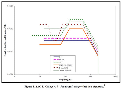
Figure 22: Typical vibration levels that jet aircraft cargo will be exposed to.
If you were developing something for the government that was going to be transported with a jet aircraft, you would be required to do some testing on your device/equipment to prove it can survive prolonged exposure to those vibration levels. Most shaker control systems will have these exposure profiles built in but they can also be constructed easily given some known PSD levels and rise/decline rates. Let’s take a look at some data captured by a Slam Stick X when it was being excited with these vibration levels; all this data is available to download.

Figure 23: Raw acceleration data from Slam Stick when exposed to random jet aircraft cargo vibration levels.
Obviously the raw data in the time domain doesn’t tell us much although the amplitude of the vibration in the time domain of nearly 20g is surprising. Let’s compute both FFTs and PSDs of these signals to see how the signal length affects the amplitude for the FFT but not the PSD.

Figure 24: The amplitude of the PSD doesn’t change with different signal lengths but the FFT does.
The red lines in the PSD are the input error bounds that the shaker is trying to keep the signal within. As you see, the PSD of different signal lengths just fills in this area but the amplitude doesn’t change overall. The FFT amplitude however shifts down as the bandwidth is increased. This normalization that occurs in a PSD calculation makes it so much more desirable to be used when analyzing random vibration signals.
Now let’s put ourselves in the shoes of someone buying equipment to be integrated into a larger system. We will want to make sure this equipment can handle the vibration levels in this environment so we may require a test organization to quantify that environment. A Slam Stick recently recorded data on a commercial flight to do just this; its aim was to understand the type of vibration levels humans were exposed to during flight. Check out the data below along with a PSD (again this is all available to download).

Figure 25: Random vibration levels on the seat of a commercial airliner.
There is definitely a resonance of that seat around 250 Hz; but there is surprisingly steady broadband vibration of 10-5 g2/Hz from 1 Hz to 1 kHz. This PSD could be used to program an exposure profile in a laboratory shaker to allow an engineer to do some in-house testing ahead of a field test. Because this was from actual data in the actual environment, the engineers have confidence that their system can survive. It’s incredibly valuable to go out and actually measure the environment than to simply rely on some test standard. These test standards will recommend using the standard’s data as a guide; but they typically try and encourage the engineer to go out and get the actual vibration data. Nothing beats the real data!
The vibration response spectrum (VRS) is used to quantify how a system will respond for a given vibration input. It takes the vibration input, in the form of a PSD, and plots what the response will be as a function of a system’s natural frequency. The vibration response spectrum calculates the transmissibility functions for a range of frequencies. Engineers use this in the design process to understand what natural frequencies to avoid or target for their system.
Let’s use the airplane seat vibration data as an example. If we were an engineer designing a component for that seat, like the personal video screen, we would need to understand what natural frequencies to avoid. Taking a look at the raw data and the PSD (Figure 26) it’s obvious that 250 Hz should be avoided; but how bad would a system with that natural frequency respond in that environment?

Figure 26: The raw data and a corresponding power spectral density are shown for 10,000 data points recorded with a Slam Stick on the base of a commercial airplane seat.
Using the MATLAB GUI package on Tom Irvine’s vibrationdata blog the transmissibility ratio for a 250 Hz single-degree-of-freedom system can be calculated, shown in Figure 27. This assumes the system has a quality factor (Q) of 10. The response of such a system would amplify the vibration amplitude by 100 times! The overall RMS vibration level of a 250 Hz is nearly 0.8g RMS compared to the 0.1g RMS level of the base vibration. That’s a significant increase in the vibrational environment that the screen would have to survive.

Figure 27: Transmissibility of 250 Hz SDOF system with the airplane seat input vibration profile is shown on the left. The corresponding power spectral density of such a system in that environment is shown on the right.
What about other frequencies besides 250 Hz; how would those systems respond? That’s where the vibration response spectrum comes in; it calculates the response acceleration (measured by RMS) for a range of natural frequencies as shown in Figure 28. It also uses a Rayleigh distribution to determine the n-sigma peak to use as a safety factor during the design process.

Figure 28: The vibration response spectrum for the airplane seat data calculates the response for different natural frequencies of a candidate system.
From the vibration response spectrum the engineer knows to either us some isolator mounts with a natural frequency below 100 Hz to dampen the vibrations or a stiff mount in excess of a couple hundred hertz natural frequency to at least not amplify the vibration levels in the environment.
Let’s take this example a step further and develop a test standard PSD from the experimental data. That data that was captured with the Slam Stick represents actual data; but can a simplified PSD be developed off that experimental data? Again using the MATLAB GUI package, a simplified PSD can be created that envelopes the maximum expected flight level plus some margin. This is a more prudent approach because conditions experienced experimentally may vary in the future (the weight of the passenger in the seat, temperature in the cabin, engine speed etc.). Using a trial-and-error approach the script derives the least possible PSD that meets the VRS requirement of the raw data shown in Figure 29.

Figure 29: An enveloped PSD is calculated using a vibration response spectrum to ensure it meets or exceeds the VRS of the experimental data.
The vibration response spectrum of the simplified PSD is shown in Figure 30. It still envelopes the same levels as that shown in Figure 28; but it does so more conservatively. This PSD may be distributed to customers so that they can design their components accordingly and test them to appropriate vibration levels. Note the relative displacement shown in Figure 30; if isolator mounts are used then it’s important to ensure they can withstand the expected relative displacement levels so they don’t bottom out.

Figure 30: The vibration response spectrum of the simplified PSD is shown along with the relative displacement.
Tom Irvine’s 16th webinar goes through the vibration response spectrum in much more detail and is a great reference if interested in the vibration response spectrum. More detail is available on his VRS tutorial.
Similar to the vibration response spectrum, a shock response spectrum is used to calculate the response for a given shock excitation. The math and use case is very similar in both instances; it enables the engineer to design his/her system avoiding certain natural frequencies that would amplify the shock input.
Let’s look at an academic example of designing a system to survive a 1g, 1 second half sine pulse. We’ll explore the response from seven different resonant frequencies (and corresponding spring stiffness) ranging from 0.063 Hz to 4.0 Hz. The system is shown in Figure 31, this information is all taken from the vibrationdata SRS educational animation page.

Figure 31: A seven spring system is shown with natural frequencies increasing by a power of 2 between each other.
Figure 32 shows six frames of the response out of these springs as they experience the shock input. The full video is available to download on Tom Irvine’s vibrationdata page. One can see the spring on the far left experience very little overall motion but it had to withstand a significant amount of relative motion and spring compression. On the far right the spring tracks the base input with very little spring compression. The middle systems experience widely oscillating acceleration throughout the input and then after the shock impulse has ended.

Figure 32: From top left to bottom right the frames are spaced approximately 0.25 seconds apart as the base input goes through a 1 second half sine pulse.
Using the MATLAB GUI package on Tom Irvine’s vibrationdata blog we can calculate the response out of these systems shown in Figure 33. Notice how the stiffest spring tracks the input nicely and then quickly rings out after the base excitation is done. The softer springs also oscillate after the base input is finished but they do so much more slowly and experience their maximum acceleration levels when the input is already finished. Figure 34 plots the relative displacement the springs need to endure during the event and afterwards; this illustrates that if you go the route of a damper, you need to ensure it has enough spring compression available for your environment.

Figure 33: Response from different springs for the given base input of 1g, 1 second half sine pulse.

Figure 34: The absolute value of the relative displacement between the masses and the base input is plotted on a logarithmic scale to illustrate the much larger spring compression that the softer springs need to endure.
Instead of testing each spring, a shock response spectrum can be used to calculate the response for a range of natural frequencies, plotted in Figure 35. This plot can be used by the design engineer to determine frequencies that should be avoided in his/her design. This example is an academic one but even so, an engineer may be surprised that for a 1 second half sine input, the worst natural frequency a system could have is around 0.8 Hz, not the 0.5 Hz of the input. In real world applications you will have real test data that will have many frequency components. As always with these analyses; your analysis can only be as good as the raw experimental/input data.

Figure 35: The shock response spectrum is shown for a 1g 1 second half-sine pulse input.
Tom Irvine’s 23rd webinar covers the classical shock pulse and the shock response spectrum if you are interested in more information. Beyond the more basic shock response spectrum, a look at the pseudo velocity shock response spectrum may be a prudent exercise if/when designing a system to survive shock.
Modal analysis is the logical next step of vibration testing and looking at response spectrums; it allows the engineer to determine key dynamic parameters of their structure:
- Modal resonant frequency
- Modal damping
- Mode shape
Picture a flat plate supported in the center with an accelerometer positioned in one of the corners. Then excite the plate with a sinusoidal sweep of different frequencies but fixed amplitude and measure the response from the accelerometer. If you do this an accelerometer may measure the type of response shown in Figure 36. You may expect that the output from the accelerometer would also be fixed because of the fixed input levels; but this is the whole beauty of modal analysis! The response amplifies as the force is applied with a rate of oscillation closer to the resonant frequencies in the system.

Figure 36: Response from accelerometer on a plate measuring acceleration as the plate is excited with a range of different frequencies, but a fixed force amplitude.
If a frequency response function is applied to the data the resulting plot is a function of frequency shown in Figure 37. This allows the engineer to directly see where the resonant frequencies lie but with curve fitting, you can also determine the damping characteristics of each mode.
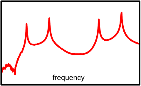
Figure 37: Frequency response function from a modal analysis test.
If a grid of accelerometers are placed around the plate and the same exercise is repeated, you can begin to start seeing modal shapes at each one of these resonant frequencies. The first four modes of this representative plate are shown in Figure 38: a first bending mode, a twisting mode, the second bending mode, and a second twisting mode. For an interesting video on the modal shapes of a plate, check out this video.

Figure 38: Mode shapes emerge at each resonant frequency which provides more information on the dynamic characteristics of your structure.
Understanding a structure’s mode shapes help the engineer better design his/her structure. Performing experimental modal analysis also helps the engineer correlate or validate a finite element model so that they can have more confidence in their design and optimize it for a particular operational environment.
Modal analysis is a very powerful tool but it typically requires a fairly expensive and complex test setup (many wired accelerometers, a shaker and/or impact hammer, large data acquisition system, and a powerful software package). So it has its limitations and is traditionally reserved for expensive and/or large structures for testing and design; a typical design engineer for a smaller or lower volume product/system may not be able to afford this type of analysis and testing.
For hardware and software, m+p International seem to offer some of the best that we’ve come across but there are other options too. Typically though, a modal analysis setup will cost tens of thousands of dollars. But the information it provides is arguably easily worth the cost for some applications!
If you are interested in finding out more on modal analysis, check out Dr. Peter Avitabile’s Modal Space articles (the previous images are from this collection of articles). He has been doing modal analysis for 40 years and “grown up” with the industry; so finding an expert with more experience than him is very difficult, if not impossible! Brüel and Kjaer also have a two part Structural Testing document (part 1 is mechanical mobility measurement; part 2 is modal analysis and simulation). These documents were written back in 1988; but they are still applicable even today, especially the fundamentals. The most thorough and modern resource we’ve come across is available from the Modal Shop, The Fundamentals of Modal Testing.
Shock and vibration testing in the field is a great way to get operational data on your system’s response to its environment and/or to quantify the environment you intent to operate in. But as the design process advances and prototypes are constructed it will be advantages to do some controlled shock and vibration testing in the laboratory. There are a couple main purposes of laboratory testing:
- Qualification testing
- During design process
- To meet test or regulatory standards
- Fatigue testing
- Modal analysis
- Evaluating performance characteristics
There are two main types of vibration shakers/exciters for general shock and vibration testing: electrodynamic (ED) and hydraulic. Figure 39 provides a plot comparing the operating ranges of these two types of exciters. Electrodynamic is much more common because of the wider frequency range, their linear behavior, and their wide range of operating conditions (shock and SRS pulses in addition to vibration). But for maximum displacement and lower frequency ranges a hydraulic shaker would be preferred.

Figure 39: The useful operating regions of hydraulic and electrodynamic vibration shakers. This plot is from the Brüel and Kjaer’s Mechanical Vibration and Shock Measurements. This book was published in the 80s so the performance ranges have changed since then slightly; but this data is still effective at highlighting the difference between the two types of vibration shakers.
At Midé we use a Brüel and Kjaer electrodynamic shaker for our shock and vibration testing, including calibration of our Slam Stick data loggers; specifically we have the LDS V455 permanent magnet shaker shown in Figure 40. There are other companies that sell shakers such as Data Physics, and Unholtz-Dickie. The trouble with buying these larger general purpose shakers in your company’s lab is the typically high costs they require. These type of industrial shakers will cost tens of thousands of dollars and that doesn’t include the high cost of the amplifier and software to run the shaker (tens of thousands for these too).

Figure 40: The LDS V455 is a good general purpose shock and vibration shaker. It has a useable frequency range of 5 Hz to 7.5 kHz, a peak-to-peak displacement maximum at 0.375”, and a maximum sine force peak at 100 pounds-force.
Shakers are also used extensively in modal testing. In these test setups, typically a much smaller shaker is needed to excite the range of modal frequencies you may be interested in. For this type of testing the Modal Shop offers the best range of solutions, including rental services. Figure 41 provides an image and performance plot of one of their mini-shakers. This shaker is ideal for general purpose testing on small components and also very useful as an excitation source for modal testing.

Figure 41: The Modal Shop’s 2004E mini-shaker is pictured with its payload curve.
Their shakers may also work as general vibration and shock exciters for smaller systems to qualify your product/design as shown in Figure 42; but their equipment is best suited for smaller test setups and/or modal testing.

Figure 42: The Modal Shop’s general purpose vibration shakers performance range is dependent on payload mass and maximum acceleration levels desired.
Another form of exciting your structure for the purpose of modal testing is using an impact hammer. These offer a much more cost effective means of performing your testing (a typical impact hammer will cost just under $1,000) and are the preferred method for many experts. An impact hammer will provide a nearly constant force over a broad range of frequencies (specified by the type of tip you use); and therefore these are capable of exciting a broad range of resonances and modal shapes. These hammers will come force-instrumented so that the frequency response function can be calculated using output of modal accelerometers instrumented throughout your structure.
Figure 43 provides some performance specifications of one of PCB Piezotronics’ impact hammers that cost $760. The Modal Shop (owned by PCB) also offers a variety of impact hammers which can be purchased or rented.
Figure 43: PCB’s model 086C03 impact hammer and its performance is shown.
Performing shock and vibration testing in a simulated environment can be very expensive and require complex equipment and setups. But there are test laboratories that can offset some of these costs (although their services will still be several thousand dollars). Midé has had experience with both National Technical Systems (NTS), and Dayton Brown. For larger systems, like those being qualified for naval ships, Hi-TEST laboratories offers shock and vibration testing services. This includes their MIL-S-901D shock testing capabilities that consist of exploding a charge underwater to subject a test setup to a large displacement shock event. Midé has been down there a couple times for our bulkhead shaft seal and stern tube seal product lines as well as for some of our general R&D programs. It is both exciting and nerve racking to witness those tests!
Setting up test hardware and knowing what/how to analyze the vibration data is meaningless without the means to perform that analysis. Software is also typically needed to acquire the vibration data in the first place. There are a wide variety of software packages available to the test engineer but he/she needs to answer two questions before settling on a software option or combination of options:
- Do you need to analyze data in real-time, or post-process the shock and vibration data?
- Do you prefer developing your own analysis and simulation programs, or using a standalone graphical user interface?
If the products you will be using acquire the data and export it then the software will “only” need to do the post-processing. This would be the case for a data logger. But for applications that require real-time (or near real-time with a buffer) data streaming and analysis will limit the options available. Real-time data streaming and processing is needed for typical modal analysis, and for controls applications (where an action is taken based upon recorded data).
Writing custom analysis and simulation programs will require some advanced knowledge of the computing language and analysis fundamentals; but is the preferred path for most post-processing analysis applications. Standalone graphical user interfaces (GUIs) are nice for providing that initial overview of your data and performing some analysis. In many applications though there will be a need for doing analysis based upon certain conditions specific to your test. For example, if I performed a two hour long test on an aircraft component, I may want to develop a script that looks through the data and runs FFTs if/when certain conditions are met. Doing this fairly simply analysis that has a couple if-statements may be more difficult in a standalone GUI.
Most times a combination of standalone GUIs and custom analysis scripts will offer the best of both worlds to complete your analysis. There are a lot of options out there but it can be difficult to go through and compare them. Below we’ve condensed the list to a few more well-known software packages.
MATLAB is a programming language specifically developed for linear algebraic operations. Because of this initial core design and focus, it is a hugely popular tool for data analysis. Engineers would have used MATLAB is college and entered the workforce already with a knowledge and preference for this (MathWorks is smart with their pricing to offer significant discounts to universities and students).

Figure 44: MATLAB is the most common programming tool used by vibration analysts.
The big disadvantage of MATLAB is that it's not free; a commercial license will cost $2,150. They also charge more, typically $1,000, for additional toolboxes (here's a full price list of the MATLAB products); and I'd recommend the signal processing toolbox for vibration analysis. Don't worry though, I didn't use any functions in that toolbox for this analysis or the ones covered in my vibration analysis basics blog.
If code base programming seems daunting, MATLAB does have their Simulink block diagram environment. This is a compelling product that can help reduce human programming induced errors and allow teams of analysts to integrate their algorithms a little easier. A single commercial license is $3,350 (in addition to a MATLAB license). Simulink also lets engineers interface with hardware such as National Instruments, Raspberry Pi and Arduino; but these hardware supports will cost you. Simulink is great for analyzing data in real time (another couple thousand dollars) and offers incredible customization in addition to built-in analysis capabilities.
Python is a free, open source, and very versatile programming language. Their NumPy and SciPy packages have similar functions to MATLAB. Python is a pretty elegant and intuitive programming language compared to MATLAB. It was created to be a generic language that is easy to read; and they definitely succeeded with that! Python is universally accepted as the better alternative to MATLAB for other programming needs besides data analysis.
But if you ask what’s better, MATLAB or Python for vibration analysis, you may start a heated debate because they both have benefits and disadvantages. We recently did some testing to compare MATLAB and Python for vibration analysis and came to the conclusion that for basic analysis (including FFTs) Python can match and even beat MATLAB computation times; but the programmer may need to do a bit of digging to find and download all the necessary libraries. But these libraries will be free!
As a MATLAB user I found the Anaconda distribution of Python and its most popular libraries very helpful. The Spyder development environment, shown in Figure 45, has a similar interface and feel to MATLAB for those with MATLAB experience.

Figure 45: The Spyder Python development environment is shown; it has a similar interface to MATLAB.
Python is gaining popularity because it’s free and the community is generating a wide variety of versatile libraries that are publically available through GitHub. A quick search finds the PyDAQmx library that interfaces with National Instrument’s drivers. Again Python is free so it’s becoming a compelling alternative, especially as they offerings and capabilities continue to grow and improve.
Most engineering companies will likely have a couple LabVIEW licenses to interface with their National Instruments data acquisition hardware and analyze data in real time. LabVIEW is a development environment specifically designed for engineers and scientists analyzing data. As such, it’s a popular tool for vibration testing! As we’ve discussed, National Instruments is the world leader in hardware for data acquisition; so it makes sense that their software is also very popular and pairs well with their hardware. Designing analysis programs with LabVIEW may be easier to those with less programming knowledge because of the graphical programming language they use, shown in Figure 46.

Figure 46: LabVIEW’s block diagram design environment is shown next to a representative analysis window.
A full LabVIEW license costs $2,999 and vibration customers may be interested in their Sound and Vibration Toolkit for another $1,999. It can definitely get expensive quickly but is a great solution for data analysis, especially in real-time controls applications.
There are a wide range of standalone software packages available for purchase; but let’s first identify a couple free ones.
Tom Irvine offers both a MATLAB and Python version of his signal analysis and structural dynamics software GUI. These offer great versatility because it has a nice GUI which is easy to work with; but all the source code is available if you need to take the next step and perform your own custom analysis. In nearly all of his webinars he will go through an example that uses these software packages so you can quickly see the power and ease of use of these analysis options.

Figure 47: Vibrationdata’s MATLAB signal analysis GUI window is shown with a broad range of analysis capabilities.
Midé’s Slam Stick Lab is available for free along with some example recording files. This software currently only works with Slam Stick recording files; but Midé has plans to open this up to other import files in the future. The software only has basic analysis capabilities but it covers the major ones typically needed: FFT, PSD, spectrogram, unit conversion, and general plotting. Data can be exported to MATLAB or CSV (readable by Excel, Python, and other software) for follow on analysis.

Figure 48: Slam Stick Lab software is a free standalone GUI for analyzing Slam Stick vibration logger recorded data.
The following represent a select few of many different standalone GUIs available on the market for vibration analysis. These will typically cost around $5K or more but offer some unique benefits over writing your own code, namely a time savings advantage.
This company specializes in vibration testing, specifically modal. They have a variety of hardware products for data acquisition but also some software packages for post processing and analyzing data in real-time. Their m+p analyzer can interface with their hardware for real time analysis but is also useful in handling large datasets and post processing vibration data.
Vibration Research’s VibrationVIEW software is another alternative to post processing and analyzing vibration data in real time.
Bruel and Kjaer have a couple different software packages that are very impressive; again for both post processing and analyzing vibration in real time.
Xcitex’s ProAnalyst software is unique in that it uses video for determining vibration levels and analyzing them. Seems like a very powerful tool that can simplify the hardware setup! The costs don’t seem too ludicrous either, only $1,795 for their introductory edition. It quickly starts climbing towards $10K and beyond though for the professional edition and different toolkits. I do like how they come right out and list the pricing instead of requiring you to fill out a form!
For modal analysis and validating CAD models with experimental data, FEMtools is a very powerful tool. It can also be used for general post processing of time history vibration data.
Before you can dive into vibration measurement and analysis it’s important to ask yourself and answer those first couple questions: what frequency and amplitude is of interest, who needs the data and why, where is the test environment, when is the testing, and when does the analysis need to be completed by?
Remember that shock and vibration testing is an art and a science. It’s not always very straightforward; but that creates some opportunity as the engineer to impart their own personality into testing and analysis. It lets the engineer have fun, so go out and have fun with your vibration testing!

Here is a case study of how the US Navy used one of our portable Slam Stick data loggers to locate a source of cockpit vibration in a C-2A Greyhound Aircraft.
Avitable, Peter. Modal Space (in our own little world). 2014. Web.
Broch, Jens Trampe and Joëlle Courrech. Mechanical Vibration And Shock Measurements. Naerum, Denmark: Brüel & Kjaer, 1980. Print.
Harris, Cyril M and Allan G Piersol. Harris' Shock And Vibration Handbook. New York: McGraw-Hill, 2002. Print.
Irvine, Tom. Shock and Vibration Signal Analysis. 2005. Web. 12 September 2005.
McConnell, Kenneth G. Vibration Testing. New York: Wiley, 1995. Print.
Technical Papers