
- Home
- Shock & Vibration Resources Center
- Handbooks
- Bernoulli-Euler Beams

Beam Equations


The governing equation for beam bending free vibration is a fourth order, partial differential equation.

The term  is the stiffness which is the product of the elastic modulus and area moment of inertia. The equation for a uniform beam is

The method of separation of variables can be applied as


Substitution into equation (1.2) leads to spatial ordinary differential equations

Define the wavenumber β as

The differential equation can be expressed as

The spatial solution has the form

Substitute the spatial solution into the differential equation.

Equation (1.10) is satisfied by the wavenumber relationship in equation (8.7), which gives credibility to the assume spatial solution. The  values in equations (1.9) and (1.10) are coefficients that depend on the boundary conditions discussed in 8.1.2. The spatial solution gives eigen function modes shapes. It also gives eigenvalue roots from which the natural frequencies are calculated.
The eigenvalues are represented as  . The angular natural frequencies
  are
are

Common Boundary Conditions
Recall the cantilever or fixed-free beam in Figure 1.1. The displacement and slope at the fixed end are both zero.

The moment and shear force at the free end are both zero.


Application of these boundary conditions to the spatial displacement in equation (1.9) and its derivatives yields the following equation for finding the  coefficients.

By inspection, equation (2.4) can only be satisfied if  and
and  . Set the determinant of the matrix to zero in order to obtain a nontrivial solution. This yields the following transcendental equation for finding the roots by the Newton-Raphson method. There are multiple roots which satisfy equation. A subscript is thus added.

The fundamental root for the cantilever beam is  . The natural frequencies can be found by substituting each root in to equation (1.11).
Recall the pinned-pinned beam in Figure 1.2. The boundary conditions at the left end of the pinned-pinned beam are

The boundary conditions at the right end are similar.
Application of these boundary conditions to the spatial displacement in equation (1.9) and its derivatives yields the following equation for finding the coefficients.
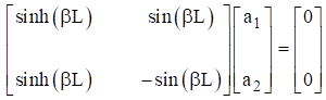
By inspection, equation (2.4) can only be satisfied if and . Set the determinant of the matrix to zero in order to obtain a nontrivial solution. This yields the following transcendental equation. There are multiple roots which satisfy equation. A subscript is thus added.

The equation is satisfied if

The natural frequencies can be found by substituting each root in to equation (1.11).
The solutions to the beam equation for various boundary conditions are derived in Reference [7]. A summary of beam formulas is given in Table 3.1. Note that the free-free beam also has a rigid-body mode with zero frequency.
| Configuration | Fundamental Frequency |
|---|---|
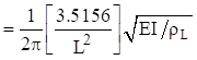
| Cantilever (Fixed-Free) |  |
| Cantilever with end mass |  |
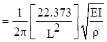
| Pinned-Pinned | 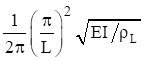 |
| Free-Free & Fixed-Fixed |  |
| Fixed-Pinned | 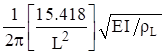 |
The pinned-pinned beam has integer harmonics as follows.

The beam bending frequencies for other configurations have non-integer harmonics. The free-free beam higher modal frequencies are shown in Table 3.2. The free-free formulas also apply to the fixed-fixed beam. The fixed-free beam higher modal frequencies are shown in the following table.
| Mode | Natural Frequency (Hz) |
|---|---|
 |
 |
 |
 |
 |
 |
 |
 |
| Mode | Natural Frequency (Hz) |
|---|---|
|
 |
|
 |
|
 |
|
 |
Again, the mode shapes  and their corresponding mode shapes are found by applying the boundary conditions to the displacement shape in equation (1.9). The participation factors are then

The effective modal mass is


Both the red and blue circles oscillate in the vertical axis in the above figure. The red circle travels at the phase velocity. The blue circle propagates twice as fast at the group velocity and is always at or near the positive or negative peak in the wave packet. The phase speed is the more important of the two speeds for vibroacoustics analyses where the bending waves are excited by the external sound field, or vice versa.
Bending waves are dispersive as a result of the governing fourth-order partial differential equation. The wave speed varies with the angular natural frequency. The phase speed for a given frequency is

The group speed is twice the phase speed.

Demonstrating bending wave propagation in terms of these two speeds is best done with an animation, but the still images in Figure 5.1 may be useful. Furthermore, the phase speed is related to the frequency and bending wavelength by

Natural frequency and modes shapes can also be derived from a beam’s energy terms via the Rayleigh-Ritz or finite element method. The following formulas are given for reference. The total strain or potential energy of a uniform beam is

The total kinetric energy  of a uniform beam is


The area moment of intertia is

The mass per length is

The natural frequency is

The tallest wind chime was struck separately from the others. The resulting sound was recorded and analyzed. The sound tone represented bending modes. The theoretical value from equation (7.3) agrees closely with the measured frequency 244 Hz. A comparison of the first four bending modes and their respective theoretical values from Table 3.2 is given in Table 7.1. There are two orthogonal planes where transverse vibration occurs. Each mode actually represents a pair of modes. The pair should ideally have the same frequency but may be slightly different due to manufacturing and material imperfections, as well as two holes in each for the connecting cord.
| Mode | Calculated (Hz) | Measured (Hz) | Musical Note |
|---|---|---|---|
| 1 | 238 | 244 | B |
| 2 | 657 | 664 | E |
| 3 | 1288 | 1273 | D# |
| 4 | 2127 | 2050 | C |

The Y-axis represents transverse displacement which has been normalized to have a maximum absolute value of one. The points where each curve crosses the zero baseline are nodal points.

The time history shows some beat frequency effect because each mode is really a pair of orthogonal modes with closely-spaced frequencies.

The highest response is at the fundamental bending mode at 244 Hz. The fourth bending modes at 2050 Hz is barely excited. Note that Fourier transforms are covered in Section 15.
