

- Home
- Shock & Vibration Resources Center
- Handbooks
- Digital Filtering

Filtering Introduction
Filtering is a tool for resolving signals. It can be performed on either analog or digital signals. Analog anti-aliasing filtering was covered in Section 14.4. The present section is limited to digital filtering with an emphasis on the Butterworth filter, which is implemented in the time domain as a digital recursive filtering relationship.
High-pass & Low-pass Filters
A high-pass filter is a filter which allows the high-frequency energy to pass through. It is thus used to remove low-frequency energy from a signal.
A low-pass filter is a filter which allows the low-frequency energy to pass through. It is thus used to remove high-frequency energy from a signal.
A band-pass filter may be constructed by using a high-pass filter and low-pass filter in series

A Butterworth filter is one of several common infinite impulse response (IIR) filters. Other filters in this group include Bessel and Chebyshev filters. These filters are classified as feedback filters. The Butterworth filter can be used either for high-pass, low-pass, or band-pass filtering. It is characterized by its cut-off frequency. The cut-off frequency is the frequency at which the corresponding transfer function magnitude is –3 dB, equivalent to 0.707. The transfer function curves in Figure 20.1 each pass through the same cut-off frequency point.
A Butterworth filter is also characterized by its order, with the sixth-order preferred in this document. A property of Butterworth filters is that the transfer magnitude is –3 dB at the cut-off frequency regardless of the order. Other filter types, such as Bessel, do not share this characteristic.
Consider a lowpass, sixth-order Butterworth filter with a cut-off frequency of 100 Hz. The corresponding transfer function magnitude is given in Figure 20.2.
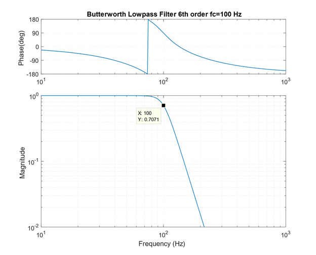
Note that the curve in the above figure has a gradual roll-off beginning at about 70 Hz. Ideally, the transfer function would have a rectangular shape, with a corner at (100 Hz, 1.0). This ideal is never realized in practice due to stability concerns in the time domain. Thus, a compromise is usually required to select the cut-off frequency. The transfer function could also be represented in terms of a complex function, with real and imaginary components. A transfer function magnitude plot for a sixth-order Butterworth filter with a cut-off frequency of 100 Hz as shown in Figure 20.3.
The curves in the previous figure suggests that filtering could be achieved as follows:
- Take the Fourier transform of the input time history
- Multiply the Fourier transform by the filter transfer function, in complex form
- Take the inverse Fourier transform of the product
The above frequency domain method is valid. Nevertheless, the filtering algorithm is usually implemented in the time domain for computational efficiency, maintaining stability, avoid leakage error, etc.

The filter transfer function can be represented by H(ω) as shown in Figure 20.4.
The filtering transfer function is implemented as a digital recursive filtering relationship in the time domain. The response  at time index
  is
is

The filter order is  The filter coefficients
  and
and  can be derived using the method is Reference [42]. The equation is recursive because the output at any time depends on the output at previous times.

An ideal filter should provide linear phase response. This is particularly desirable if shock response spectra calculations are required. Butterworth filters, however, do not have a linear phase response. Other IIR filters share this problem. Methods are available, however, to correct the phase response. One is the refiltering method in Reference [42]. An important note about refiltering is that it reduces the transfer function magnitude at the cut-off frequency to –6 dB, as shown in example in Figure 20.6.

Recall the synthesized time history from Figure 16.10 which satisfied the Navmat P-9492 PSD specification. Calculate the power spectral density by applying band-pass filtering over successive bands. This method is useful as a means of better understanding the PSD function. The filtering is performed using a Butterworth sixth-order filter without refiltering for phase correction. The bands are full octave. The results are shown in the following table.
| fl (Hz) | fc (Hz) | fu (Hz) | Δf (Hz) | GRMS | GRMS^2 | GRMS^2/Hz |
|---|---|---|---|---|---|---|
| 14 | 20 | 28 | 14 | 0.36 | 0.13 | 0.0091 |
| 28 | 40 | 57 | 29 | 0.80 | 0.64 | 0.0226 |
| 57 | 80 | 113 | 56 | 1.47 | 2.17 | 0.0384 |
| 113 | 160 | 226 | 113 | 2.16 | 4.67 | 0.0413 |
| 226 | 320 | 453 | 227 | 2.92 | 8.54 | 0.0377 |
| 453 | 640 | 905 | 452 | 3.11 | 9.70 | 0.0214 |
| 905 | 1280 | 1810 | 905 | 3.02 | 9.15 | 0.0101 |
| 1810 | 2560 | 3620 | 1810 | 1.31 | 1.71 | 0.0009 |
The band center frequency is fc. The lower and upper band limits are fl and fc, respectively. The bandwidth is Δf which is the difference between the band limits. A GRMS value is calculated for each band. Then the GRMS value is squared and divided by the bandwidth. The last column is the PSD in GRMS^2/Hz. The time histories for the two rows in the table are shown in Figure 20.7. The GRMS^2/Hz points are plotted along with Navmat PSD in Figure 20.8. Recall that GRMS^2/Hz is abbreviated as G^2/Hz. The bands are in full octave format.


The PSD points calculated via band-pass filtering track the specification fairly well. The dropout for the last point is not a concern because the bandwidth extended from 1810 to 3620 Hz, but the specification stopped at 2000 Hz.
The following example shows how filtering can aid in analyzing seismic data from a seismometer. Filtering is used to find onset of P-wave in seismic time history from Solomon Island earthquake, Magnitude 6.8, October 8, 2004. The measured data is from a homemade seismometer in Mesa, Arizona.

The boom is a horizontal pendulum. It has a period of 14.2 seconds, equivalent to a natural frequency of 0.071 Hz. A sensor at the free end measures the displacement. The boom length is 64 inch. The total frame height is 35 inch. The boom has a knife edge that pivots against a bolt head in the lower cross-beam of the frame.
The boom is suspended from the frame by a wire cable. The cable is attached to the top cross-beam of the frame. The other end of the cable is attached to the boom, about two-thirds of the distance from the pivot to the free end of the boom. The pivot point is offset from the top cable attachment point. Thus, the boom oscillates as if it were a "swinging gate."
The plate supporting the frame has three adjustable mounting feet. The feet can be adjusted to tune the pendulum to the desired natural frequency. Furthermore, the wire cable has a turnbuckle which is used to adjust height of the free end of the boom. The detached frame in the center of the figure is used for assembly and to limit the displacement during tuning.

The classic sensor for Lehman seismometers is a magnetic coil attached to the boom. The coil moves between the poles of a magnet, thus inducing a voltage proportional to the velocity. The signal requires tremendous amplification. The author has better success with the inductive displacement sensor.

The damping method is shown in this figure.

The chisel blade butted up against a chrome-plated bolt head.

The seismometer was given an initial displacement and then allowed to vibrate freely. The period was 14.2 seconds, with 9.8% damping. The corresponding frequency is 0.0705 Hz.

The trace in the above figure is the displacement time history of the Solomon Islands earthquake on October 8, 2004 as measured by the Lehman seismometer via the inductive sensor. The seismometer was located at home in Mesa, Arizona. The data was acquired by a Nicolet Vison system. The Nicolet sample rate was set to 50 samples per second with its lowpass filter set to 5 Hz.
A Krohn-Hite filter, model 3343, was used to high-pass filter the analog displacement signal at 0.03 Hz prior to its input to the Nicolet system. It also provided a 20 dB gain.
The time is referenced to the earthquake occurrence using the USGS data. The plot’s Y-axis is labeled as relative displacement because it is the response of the boom relative to the ground. Further calculation would be required to estimate the true ground motion. The time history shows that the Earth is remarkably reverberant. The oscillations last well over one hour. The phase components are P primary wave, S secondary or shear wave, and LQ Love wave. Recall the seismic wave diagrams in Section 18.6.1.
The P-wave is indiscernible against the background microseismic noise. Nevertheless, it can be extracted by additional filtering, as shown in the next figure.

The P-wave arrives at in Mesa, Arizona about 760 seconds after it was generated near the Solomon Islands. The S-wave arrives around 1400 seconds. There are also some intermediate waveforms which begin as P-waves and transform into other types through reflection and refraction. Both the P and S-waves are body waves which travel faster than surface waves. The frequency content of body and surface waves is shown in the following table, as taken from Reference [43].
| Wave Type | Period (sec) | Natural Frequency (Hz) |
|---|---|---|
| Body | 0.01 to 50 | 0.02 to 100 |
| Surface | 10 to 350 | 0.003 to 0.1 |
There are occasional needs to integrate accelerometer time histories to velocity. This may be done to evaluate the accuracy of pyrotechnic shock data where the velocity is expected to have a stable oscillation about its zero baseline. Accelerometer data may also be double-integrated to displacement, but the accuracy depends on the frequency response of the accelerometers. Some accelerometer types such as variable capacitance and servo motor designs can accurately measure acceleration down to zero frequency. The common piezoelectric accelerometer may have a practical lower limit of a few Hertz, however. Some type of high-pass filter is needed in this case. The high-pass filtering may be performed using an analog filter in the accelerometer’s signal conditioner. Or the filtering may be performed digitally as a post-processing step.
Another integration scenario is the case where an acceleration time history is synthesized for use in a modal transient analysis. The corresponding velocity and displacements should each be stable, especially if dynamic stresses are to be calculated. Consider the simple case of the synthesized white noise acceleration time history in Figure 20.16.
The integration steps are performed using the trapezoidal method, which has sufficient accuracy. The resulting velocity displacement each has a drift. These effects arise in part because the integration does not account for initial velocity and initial displacement, each of which are either unknown or unspecified. The next task is to correct the acceleration time history so that its velocity and displacement will each be stable. There is no one right way to do this, but an example is shown in Figure 20.17. The correction steps were:
- Remove mean from acceleration
- High-pass filter acceleration at 6 Hz, Butterworth 6th order with refiltering for phase correction
- Apply fade in and out to acceleration using 2% of the total duration at each end
- Integrate to velocity
- Remove mean from velocity
- Apply fade in and out to velocity using 2% of the total duration at each end
- Integrate to displacement
- Perform first-order trend removal on displacement
- Apply fade in and out to displacement using 2% of the total duration at each end
- Differentiate displacement to velocity
- Differentiate velocity to acceleration Integrate corrected acceleration to velocity
- Integrate velocity to displacement
- Verify that the resulting velocity and displacement each have stable oscillations about their respective zero baselines and that each begins and ends at zero


Nine subplots appear as follows:
Row 1, Col 1 - processed acceleration prior to integration
Row 2, Col 1 - integrated velocity
Row 3, Col 1 - double integrated displacement
Row 3, Col 2 - double integrated displacement (repeated)
Row 2, Col 2 - differentiated velocity from double integrated displacement
Row 1, Col 2 - double differentiated acceleration from double integrated displacement
Row 1, Col 3 - double differentiated acceleration (repeated)
Row 2, Col 3 - integrated velocity from double differentiated acceleration
Row 3, Col 3 - double integrated displacement from double differentiated acceleration
The corrected acceleration is the time history shown in Row 1, Col 2 and repeated in Row 1, Col 3.

Note that the fade in and out windows are similar to those shown in the above figure.

White noise is an idealized concept. True white noise would have a flat PSD level from zero to infinity frequency units. Digital white noise is inherently frequency limited by its sample rate. Furthermore, white noise may be subject to low-pass filtering to smooth it prior to its use as an excitation function, as shown in Figure 20.19. The top plot is a white noise sampled at 10,000 samples/sec and has a choppy appearance. Aliasing would be suspected if the top plot were measured data.
The bottom plot is the same time history low-pass filtered at 2000 Hz which smooths the data. Either time history should be suitable for either applied force or base excitation of an SDOF system with a natural frequency of 200 Hz, for example. Recall that the SDOF system itself behaves a mechanical filter. But the low-pass filtered version could have some potential numerical accuracy benefits, although an investigation of this hypothesis is left as future work.

Coupled Loads Analysis (CLA) predicts payload & launch vehicle responses due to major dynamic and quasi-static loading events. This analysis is performed prior to launch. It can also be performed as post-flight data reconstruction using flight accelerometer data. Flight accelerometer data is low-pass filtered for coupled-loads analyses. The cut-off frequency varies by launch vehicle, payload, key events, etc. The primary sources of these low frequency loads are:
- Pre-launch events: ground winds, seismic loads
- Liftoff: engine/motor thrust build-up, ignition overpressure, pad release
- Air-loads: buffet, gust, static-elastic
- Liquid engine ignitions and shutdowns
Reference [44] gives the following frequency guidelines for CLA. The low-frequency dynamic response of the launch vehicle/payload system to transient flight events is typically analyzed from 0 Hz to 100 Hz. The response frequency domain can be up to 150 Hz for some small launch vehicles.
