

- Home
- Introduction to Shock & Vibration Response Spectra

Introduction

A rocket vehicle behaves as a free-free beam during flight. The vehicle’s body bending modes can be excited by wind gusts, aerodynamic buffeting, thrust offset, maneuvers, etc. The image shows the IRVE 2 launch from Wallops Island. The vehicle is a Black Brant 9, which has a Terrier Mark 70 first stage. Flight accelerometer data showed that the fundamental bending frequency began at about 8 Hz and then swept up to 13 Hz as propellant mass was expelled. Autopilot guidance and control algorithms need to account for the body bending mode to maintain stability.

The mode shape from a finite element model is shown exaggerated. The two tines undergo an in-plane bending mode, 180 degrees out-of-phase with one another. The stem also participates in this mode, but its displacement is so relatively small that it is not apparent in the figure.
The Ancient Greek philosopher Pythagoras (570–495 BC) studied the vibration of stringed instruments and developed a theory of harmony. He first identified that the pitch of a musical note is in inverse proportion to the length of the string that produces it, and that intervals between harmonious sound frequencies form simple numerical ratios.
The ancient Greeks believed that al objects were composed of some combination of the basic elements: earth, water, air, and fire. Aristotle (384–322 BC) attempted an explanation of earthquakes based on natural phenomena. He postulated that winds within the earth whipped up the occasional shaking of the earth's surface. He noted that earthquakes sometimes caused the water to burst forth in what would now be called a tsunami.
Galileo Galilei (1564-1642) performed numerous experiments with oscillating pendulums during the Renaissance. He discovered that the period of swing of a pendulum was independent of its amplitude. He used his own pulse as a time measurement because there were no watches at that time. Christiaan Huygens (1629-1695) successfully built a pendulum clock based upon Galileo’s work.
Robert Hooke (1635-1703) developed the law of linear spring stiffness. This law has been generalized to the elasticity principle that strain in a body is proportional to the applied stress.
Sir Isaac Newton (1643-1727) derived his laws of motion, which are the foundation of mechanical vibration analysis. He published his findings in a book known by its abbreviated title Principia.
Jacob Bernoulli, Daniel Bernoulli, and Leonhard Euler derived the equation of motion for beam vibration circa 1750.
Lord Rayleigh, John William Strutt, published Theory of Sound in two volumes during 1877-1878. Volume I covered harmonic vibrations, systems with one degree of freedom, vibrating systems in general, transverse vibrations of strings, longitudinal and torsional vibrations of bars, vibrations of membranes and plates, curved shells and plates, and electrical vibrations. Volume II covered aerial vibrations, vibrations in tubes, reflection and refraction of plane waves, general equations, theory of resonators, Laplace’s functions and acoustics, spherical sheets of air, vibration of solid bodies, and facts and theories of audition.
The modern field of mechanical vibration analysis has been built upon the foundation of these authors’ works and has further developed as the result of failures and disasters, as well as the need to design, analyze and test structures and component to withstand dynamic environments. Vibration analysis is also important in other areas including semiconductor manufacturing, human exposure, energy harvesting, machine health monitoring, etc.

A Qantas Boeing 747-400 aircraft was flying from Sydney to Singapore on May 9, 2011 when the crew noticed abnormalities from the aircrafts No. 4 engine during a climb. The indications included an increase in both the exhaust gas temperature and vibration levels. The plane continued to Singapore for a safe landing and disembarkation of the passengers and crew. The Australian Transport Safety Bureau (ATSB) determined that the cause was a broken turbine blade.

A one-inch wide, four-foot long crack formed in the Washington Monument, near the top of the 555-foot obelisk, due to the Mineral, Virginia earthquake on August 23, 2011.
Railcar axles were failing under repeated “low level” cyclic stress, in the mid nineteenth century. These stresses puzzled engineers because the levels were much lower than the material yield stress. The Versailles rail accident occurred on May 8, 1842 after the leading locomotive broke an axle, and the carriages behind piled into it and caught fire causing many deaths. This prompted German scientist August Wöhler to develop the S-N curves used in fatigue analysis. The term “fatigue” was chosen to describe the “tired metal” in the axles.
The collapse of the Tacoma Narrows Bridge “Galloping Gertie” was captured on film on November 7, 1940. This failure is often referred to as the classic “resonant vibration” failure. But it was more properly a “self-excited” or “flutter” response, as discussed in Section Error! Reference source not found..
Aerospace has myriad examples of potential vibration problems. Helicopters may undergo “ground resonance” prior to takeoff. Launch vehicles may have pogo oscillations in liquid engine propulsion systems. Solid rocket boosters may have thrust oscillations. Both high performance aircraft and launch vehicles must withstand random vibration due to turbulent boundary layers and shock waves as they accelerated through the transonic velocity and encounter the maximum dynamic pressure condition.
Ships, automobiles, machine tools, buildings, nuclear reactors, and other mechanical systems and structures all have their own vibration concerns and failure modes.
There are many types of potential failure modes including yielding, buckling, ultimate stress, fatigue, fretting, fastener loosening, relay chatter, and loss of sway space. Engineers must understand these hazards so that the components, systems, and structures may be designed and tested accordingly.
Resonant excitation and is often a factor in these failures. Engineers thus have a responsibility to identify equipment natural frequencies through analysis and testing. The natural frequency is the frequency at which the system would oscillate if it were given an initial displacement and then allowed to vibrate freely. Resonance occurs when the excitation frequency is at or near the system’s natural frequency. Damping values, mode shapes, effective modal mass and other dynamic parameters are also needed for this analysis.
(https://solutions.borderstates.com/vibration-sensors-minimize-downtime/)
Machines, pumps, and other equipment with reciprocating or rotating parts may experience vibration due to blade passing frequencies, gear mesh frequencies, magnetostriction motor hum, shaft misalignment, rotating imbalance, etc. In addition, fluid handling machines, like fans and pumps will experience broadband turbulence.
Some vibration is normal. But excessive vibration may cause accelerated wear and premature failure. High vibration levels could also indicate a bearing defect. Equipment manufacturers should provide acceptable limits in terms of amplitude and frequency. The amplitude specification may be in terms of displacement, velocity or acceleration.
Vibration monitoring is thus needed to reduce maintenance costs, extend life, and improve safety. Machine vibration can be measured with accelerometers which are permanently mounted on the machine and monitored continuously with a wireless network. Or a technician may use a handheld device with an accelerometer that can be temporarily mounted to the machine via a magnetic base, as a periodic check.
Piezoelectric transducers or electromagnetic induction devices can be used to convert ambient vibration energy to electrical current to charge batteries or to power wireless sensor networks. As an example, consider a cooling pump in a factory. The pump’s vibration could be used to power its own health monitoring sensor.

(https://www.mide.com/products/vlt-9001-piezoelectric-energy-harvesting-kit)
Piezoelectric crystals are asymmetric. The asymmetry in the unit cell of the material sets up the mechanism whereby deforming the crystal leads to a small potential difference. The piezoelectric harvesters are typically cantilever beam structures. A mass may be added to the free end of the beam to tune the device to the source’s dominant vibration frequency. Note that steady vibration with a dominant frequency is best suited for harvesting. Outputs of 10 to 50 milliwatts are possible, depending on the vibration amplitude and frequency.
Another potential benefit of an energy harvesting device is that it removes energy from a system, thus providing some damping which can extend the system’s life.
There are also biomedical concerns for the case where humans are exposed to vibration. Motion sickness and seasickness may result from vibration exposure in the 0.1 Hz to 0.5 Hz domain. This may occur because the brain has difficulty processing apparently conflicting data from the eyes, ear canals, and other somatosensory organs.
Furthermore, operators of farm equipment, busses, and trains may suffer spinal damage due to long-term exposure. The human spinal column natural frequency is 10 to 12 Hz. Each organ and bodily part has its own natural frequency. Whole body vibration is addressed in ISO 2631 [1]. Hand-arm vibration is another concern for operators of power tools.
Engineers must also determine the characteristics of the shock or vibration excitation so that they can properly analyze and test the affected components or structures. Design modifications can then be made to avoid dynamic coupling between the excitation frequencies and the structure’s natural frequencies. The excitation sources can be grouped into four types.
A common example is a guitar string which is given an initial displacement and then suddenly released. Another is the Pegasus drop transient which is discussed in Section Error! Reference source not found.. An initial velocity example is a drop shock test machine.
Wind, acoustic pressure, and ocean currents impacting structures are all cases of applied force. So is footfall excitation on a pedestrian bridge. Shafts with rotating imbalance also impart an applied force within a machine. Another example is the force from a hammer striking an object. Impulse hammers are used to purposely excite a structure in modal testing to identify the structure’s natural frequencies, damping ratios and mode shapes. The force may also be applied by a small shaker attached to the structure via a stinger rod.
Seismic excitation is the classic example of base excitation. Another is an automobile traveling over a speed bump or down a washboard road. Aircraft and launch vehicle avionics components are subjected to base excitation from their mounting structures during flight. These components are tested on large shaker tables to verify that they can withstand flight vibration prior to installation into the vehicle.
Self-excited vibration is a special case where the alternating force that sustains the motion is created or controlled by the motion itself. This source type is also referred to as negative damping. Airfoil and bridge flutter are two examples in this category. See the Tacoma Narrows Bridge failure in Section Error! Reference source not found.. The pogo oscillation in a launch vehicle with liquid engines is another case.

(https://www.trailerblocks.com/blogs/trailer-blocks-blog/tagged/trailer-tech)
Ripples can form on gravel and dirt roads with dry, granular road materials. This pattern creates an uncomfortable ride for the occupants of traversing vehicles and hazardous driving conditions for vehicles that travel too fast to maintain traction and control. The resulting vibration may also damage suspension components.

The earthquake caused the Cypress Viaduct to collapse, resulting in 42 deaths. The Viaduct was a raised freeway which was part of the Nimitz freeway in Oakland, which is Interstate 880. The Viaduct had two traffic decks. Resonant vibration caused 50 of the 124 spans of the Viaduct to collapse. The reinforced concrete frames of those spans were mounted on weak soil. As a result, the natural frequency of those spans coincided with the excitation frequency of the earthquake ground motion.
The Viaduct structure thus amplified the ground motion. The spans suffered increasing vertical motion. Cracks formed in the support frames. Finally, the upper roadway collapsed, slamming down on the lower road. The remaining spans which were mounted on firm soil withstood the earthquake.

A small satellite is mounted to a slip table which is driven by a large electromagnetic shaker. The purpose of the test is to verify that the satellite can withstand the flight vibration that will be imparted by the launch vehicle.

An equipment rack is mounted via wire rope isolators to an expander head which is mounted in turn on an electromagnetic shaker.

(Image courtesy of the Modal Shop)
A small shaker applies a force excitation to an automobile fender via a stinger rod. The applied force and resulting acceleration at the input point are measured by an impedance head transducer. Response accelerometers may be mounted at various locations on the vehicle.

A thumper truck is a vehicle-mounted ground impact system which can be used to provide a seismic source to perform both reflection and refraction seismic surveys for oil, natural gas and mineral exploration. A heavy weight is raised by a hoist at the back of the truck and dropped about three meters, to impact the ground. The resulting ground waveforms are measured with geophones. Some thumpers use a technology called "Accelerated Weight Drop" (AWD), where high pressure gas is used to accelerate a heavy weight Hammer (5,000 kg) to hit a base plate coupled to the ground.

The Ku-band antenna is the disk below the lower Atlantis decal. Dither is a vibration employed in some mechanical systems to avoid stiction and to ensure smooth motion. Stiction is short for static friction. The antenna was dithered via a command signal at a frequency of 17 Hz to maintain its ability to smoothly search for Tracking and Data Relay Satellite System (TDRSS) satellites. There was a concern that the antenna’s resulting vibration would interfere with sensitive microgravity experiments such as crystal growth.

Solid rocket boosters have elongated internal combustion cavities which act as organ pipes. Vortex shedding within the hot exhaust gases drives standing pressure waves inside these cavities. These pressure waves have a fundamental thrust oscillation frequency with integer harmonics. The cavities can be modeled as closed-closed pipes because the nozzle throat diameter is relatively small compared to the cavity diameter. The Space Shuttle boosters’ thrust oscillation frequency was 15 Hz. The Ares I vehicle was projected to have a 12 Hz oscillation, but this vehicle was cancelled prior to what would have been its first flight. Note that the speed of sound in the internal hot exhaust gas is about 3500 ft/sec.

Rocket vehicles with liquid engines, such as the Titan II, may experience combustion instability, which causes excessive vibration forces. This is a potential source of self-excited vibration, whereby the elastic vehicle structure and the propulsion system form a closed-loop feedback system.
There are several types of combustion instability vibration effects. The most common effect is “Pogo,” which is similar to Pogo stick motion. In this case, a low frequency oscillation in the combustion chamber, or propellant feed system, excites the longitudinal vibration mode of the entire rocket vehicle, or some other structural mode. This may create a cyclical energy exchange between the vibration mode and the propulsion system oscillation. The problem may also be initiated when a wind gust or some other perturbation excites the vibration mode. This vibration in turn causes an oscillation in the propulsion system, which further excites the vibration.
Placing accumulators in the fuel and oxidant lines to damp out the pressure fluctuations solves this Pogo problem. The accumulator contains a volume of gas that acts like a soft spring to reduce the propellant frequency to well below that of critical structural frequencies. The accumulator volume must be carefully selected to meet this goal.

The mass value is m. The viscous damping coefficient is c. The spring stiffness from Hooke’s law is k. The displacement is x. The velocity is  . The equation of motion is derived using Newton’s law.


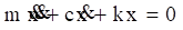
The resulting equation of motion is a second-order, ordinary differential equation, linear, homogenous with constant coefficients. The angular natural frequency in radians/sec is

The natural frequency in cycles/second or Hz is

The natural frequency is the frequency at which the system would oscillate if it were given an initial displacement and then allowed to vibrate freely. The period T is the inverse of the natural frequency.

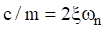
Furthermore, the damping coefficient divided by mass can be represented as
The corresponding amplification factor is

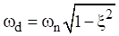
The damped natural frequency is
The free vibration solution to equation (5.3) can found using a Laplace transform and applying the initial displacement and velocity per Reference [2]. The resulting displacement is

The resulting time history is a damped sinusoid, similar to the Pegasus drop transient flight accelerometer data shown later in this document in Figure 10.7.
The conservation of energy method is based on the time derivative of the total energy of an undamped system

Apply this method to the SDOF system in Figure 5.1 to derive the equation of motion.


Dividing through by the velocity term yields the equation of motion for the undamped SDOF system.

The Rayleigh method can be used to determine the fundamental frequency of an undamped system by setting the maximum kinetic energy KE to the maximum potential energy PE.

The kinetic energy for the SDOF system in Figure 5.1 is.

The potential energy for the SDOF system is

Assume a displacement of

The corresponding velocity is

The energy terms become


Substitute the two energy terms into equation (5.15).

Algebraic simplification yields the expected natural frequency

An avionics component is modeled as a solid mass per Figure 5.1. The goal is to mount the component via elastomeric isolator bushings so that the natural frequency is 30 Hz. The isolators will filter out high frequency vibration energy from the base excitation. Calculate the required isolator stiffness using equations (5.4) and (5.5).
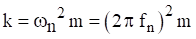

The stiffness k in equation (5.25) is the total isolator stiffness. Now assume that the component will be mounted via four isolators in parallel. The individual isolator stiffness would then be 115 lbf/in. The next step would be to determine whether isolators with that stiffness value are commercially available. Otherwise, some adjustment or compromise would be needed.
A one octave increase in frequency means that the higher frequency is twice the lower frequency. Conversely, the lower frequency is one-half the higher one. The number of octaves n between any two frequencies f 1 and f 2 is
Note that a piano keyboard has steps of one-twelfth octave counting both the black and white keys.
The octave rule-of-thumb in mechanical vibration analysis states that there should be at least a one octave separation between two frequencies to mitigate dynamic coupling. For example, consider an SDOF system subjected to a harmonic force or base excitation. The system’s natural frequency should be tuned to less than one-half or greater than twice the excitation frequency.
Isolation or low tuning would be the case where the system’s natural frequency was at most one-half the excitation frequency. High tuning occurs when the natural frequency is at least twice the excitation frequency. The system is said to be hard-mounted if the natural frequency significantly greater than the excitation frequency.
As another example, consider two SDOF systems that are to be joined together. The respective natural frequencies should be separated by on octave prior to mounting one with other. The Pegasus launch vehicle in Section 10.6 has a natural frequency of about 10 Hz. The payload’s own natural frequency should be high-tuned to 20 Hz or more to reduce dynamic coupling effects. Note that tuning below 5 Hz is a poor choice due to the possibility of high relative displacement of the payload within the vehicle fairing, as well as possible interference with the autopilot control algorithm stability. Further information about this frequency requirement can be found in the Pegasus Payload User Guide.
Complex variables with real and imaginary components are used extensively in signal analysis and structural dynamics. The imaginary component is expressed as a scale factor applied to 
Let C be a complex variable with real component A and imaginary component B.

The variable C is a vector in the complex, Euclidean plane. The magnitude is the norm.

The phase angle  is
is

Euler’s equation is a complex exponential function used for Fourier transforms and for structural modal response.

Complex exponentials can simplify trigonometry, because they are easier to manipulate than their sinusoidal components.
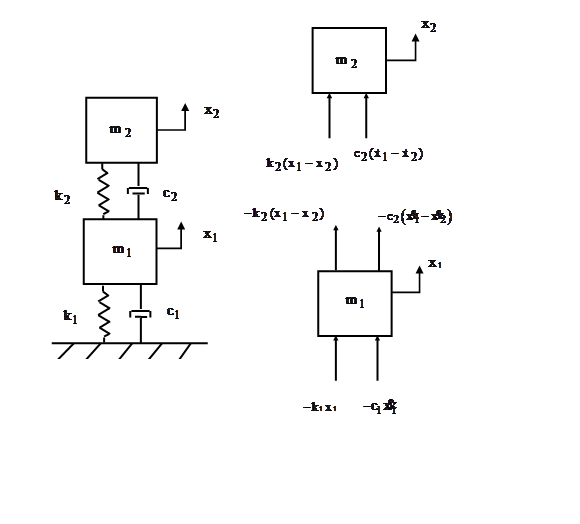
Newton’s law can be applied to the system in Figure 6.1 to derive the equations of motion. The steps are omitted for brevity. The resulting pair of ordinary differential equations can be represented in matrix form and are coupled via the damping and stiffness matrices.

A shorthand form is

The matrices and vectors are

Consider the undamped, homogeneous form of equation (6.2).

Seek a harmonic solution of the form


The  vector is the generalized coordinate vector. The undamped, homogeneous equation is transformed through substitution and algebraic manipulation into the generalized eigenvalue problem.

TThe eigenvalues  can be found by setting the determinant equal to zero.

There is an eigenvalue for each degree-of-freedom. Each angular natural frequency is then calculated from the square root of the respective eigenvalue. The corresponding eigenvectors represent orthogonal mode shapes. The eigenvector for each mode is found via

An eigenvector matrix  can be formed. The eigenvectors are inserted in column format.

The coefficient  represents the modal displacement of mass i for mode j.
Each eigenvector can be multiplied by an arbitrary scale factor. A mass-normalized eigenvector matrix  can be calculated such that the following orthogonality relations are obtained.


The superscript T represents matrix transpose. The identity matrix is I, a diagonal matrix of ones. The diagonal matrix of eigenvalues Ω.
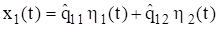
Now define a modal coordinate  in terms of the normalized eigenvector matrix such that the displacement vector is

Substitute equation (6.14) into equation (6.2).

Premultiply by the transpose of the normalized eigenvector matrix.

The orthogonality relationships yield

Furthermore, the following simplifying assumption is made for the damping matrix.

The equation of motion can now be written as

The two equations are now uncoupled in terms of the modal coordinates. The modal displacement for free vibration response to initial conditions is found via Laplace transforms as shown in Reference [3]. The modal displacement for dof i is

The damped angular natural frequency is

The physical displacement can then be found by substituting equation (6.20) into (6.14). The physical displacements can be expressed in terms of the eigenvector coefficients and modal coordinates as

The modal displacement initial conditions are required for the complete solution. These can be found from the following transformations.


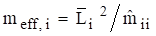
The participation factors and effective modal masses are indicators of how excitable the modes are given uniform base excitation to the given system. Some modes are more readily excited than others, and some cannot be excited at all for this excitation type.
The system’s generalized mass matrix  is given by

Again, the generalized mass will be the identity matrix if the eigenvectors are mass normalized. Let  be the influence vector which represents the displacements of the masses resulting from static application of a unit ground displacement. Define a coefficient vector
  as
as
The modal participation factor matrix for mode i is 

The effective modal mass  for mode i is
The system in Figure 6.1 has the following parameters.
| Variable | Value |
|---|---|
 |
2 lbm |
 |
1 lbm |
 |
150 lbf/in |
 |
100 lbf/in |
 |
0.01 in |
 |
0.005 in |
Assume 5% damping for each mode. The initial velocity is zero for each mass.
Apply the mass and stiffness values from Table 6.1 into equation (6.1) to form the following matrices.

The 1/386 factor is needed to convert lbm to lbf sec^2/in.
The eigenvalues and vectors are found by inserting these matrices into equations (6.9) and (6.10). The results are shown in the following table.
| Mode | Angular Natural Frequency (rad/sec) | Natural Frequency (Hz) | Participation Factor | Modal Mass Ratio |
|---|---|---|---|---|
| 1 | 125.25 | 20.0 | 0.085 | 0.935 |
| 2 | 266.72 | 42.5 | -0.022 | 0.065 |
The mass-normalized mode shapes in matrix format are
The response time histories for the initial conditions are shown in Figure 6.2.


Consider the system in the above figure. This system could represent a simple, two-node finite element model of a rod’s longitudinal vibration. A characteristic of this system is that the fundamental mode is a rigid-body mode at zero frequency. Both masses move in unison for the rigid-body mode. Newton’s law can be applied to the system to derive the equations of motion. The steps are omitted for brevity. The resulting pair of ordinary differential equations can be represented in matrix form.

The eigenvalues and vectors are found using the method shown in Section 6.1.2. Each angular natural frequency is then calculated from the square root of the respective eigenvalue.


The mass-normalized eigenvectors, representing the mode shapes, are

Again, the two masses move in unison for the first mode. They move 180 degrees-out-phase for the second mode. The semi-definite system is revisited in Section 12.3.3.
Consider the system in Figure 6.3 with the values in the following table.
| Variable | Value |
|---|---|
|
2 lbm |
|
1 lbm |
| k | 2000 lbf/in |
The mass and stiffness matrices are

The 1/386 factor is needed to convert lbm to lbf sec^2/in.
The eigenvalues and vectors are found by inserting these matrices into equations (6.9) and (6.10). The angular natural frequencies are

The mass-normalized eigenvectors in column format are
The total mass sum is 3 lbm (0.00777 lbf sec^2/in) which is also the effective modal mass of the rigid-body modes. The second mode has zero effective modal mass.

The longitudinal displacement  in a rod in undamped free vibration is governed by the second order, partial differential equation
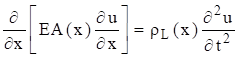
The term  is the product of the elastic modulus and cross-sectional area. The equation for a uniform rod is

Note that

Equation (7.2) is a common formula for one-dimensional wave propagation. Similar equations govern the propagation of sound in a pipe and the torsional vibration in a shaft. Note that a wave is the phenomenon in which physical energy propagates through space relative to a medium. Wave propagation is discussed throughout this document, as shown for seismic waves in Section 18.6.1 as for example.
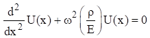
The method of separation of variables can be applied to equation (7.2) as


Substitute equations (7.4) and (7.6) into (7.2). The resulting spatial equation after some simplification is
Longitudinal waves are non-dispersive. The group and phase wave speeds are equal. The wave speed is calculated from the elastic modulus and mass density.

The speed of sound is related to the frequency and wavelength by

The spatial equation can be expressed as

The spatial solution is

The  values in equation (7.4) are coefficients that depend on the boundary conditions.
The boundary condition for a fixed left end is

The boundary condition for a free left end is

The same boundary conditions could be applied at the right end. The longitudinal natural frequencies are given in the following table.
| Configuration | Natural Frequencies | Mode Shapes |
|---|---|---|
| Fixed-Free |  |
 |
| Free-Free |  |
 |
| Fixed-Fixed |  |
 |
The mode shapes are normalized to a value of one. Note that the Free-Free beam also has a rigid-body mode at zero frequency. Further solution details are given in Reference [4]. Also, longitudinal vibration is revisited in Section 19.2.
The previous method of separation of variables is a modal solution approach. As an alternative, a wave solution can be applied to equation (7.2) as

The wavenumber  is related to the angular frequency, longitudinal wave speed and wavelength as

Natural frequency and modes shapes can also be derived from a rod’s energy terms via the Rayleigh-Ritz or finite element method. The following formulas are given for reference.
The total strain or potential energy  of a uniform rod is

The total kinetric energy  of a uniform rod is


The suspended beam can be idealized as a free-free beam for longitudinal vibration. The pendulum hammer is raised to some initial angular displacement and then released. The hammer strikes the beam’s end plate on the left end, delivering a force impulse. The longitudinal modes of the beam amplify the input energy and deliver a base input shock pulse to the test article mounted near the right end.
Bai and Thatcher described this shock test method in Reference [5]. This method is still used today, although the pendulum hammer is often replaced by a pneumatic gun firing a projectile into the beam’s end plate.
The goal was to choose the beam length so that its fundamental frequency would match the “knee frequency” of a shock response spectrum specification at 2000 Hz. (Further information on this type of specification is given in Section 18. The length for an aluminum beam to meet this goal is calculated as

Note that the longitudinal wave speed in aluminum is about 200,000 in/sec.

(https://www.enginelabs.com/engine-tech/cam-valvetrain/when-do-i-know-my-valvetrain-is-in-distress/)
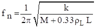
Spring surge is another form of longitudinal vibration, which arises because springs have both stiffness and inertia properties. This is in contrast to the usual simplifying assumption in vibration analysis that springs are massless. Springs used in high-speed machinery must have natural frequencies well in excessive of the frequency of motion that they control. Otherwise, the spring itself may resonate, resulting in loss of engine performance or even catastrophic failure. This can occur in automotive value springs when the engine camshaft RPM speed is increased well above the normal operating speed. Race car engines are at particular risk for this problem. Spring surge is also a potential concern when coil springs are used as isolation mounts for equipment.
The following spring natural frequencies are taken from Reference [6]. Note the similarities with the longitudinal rod formulas in Table 7.1.
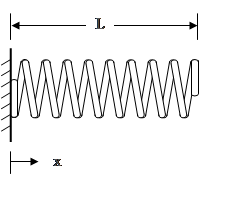
The fundamental frequency of the fixed-free spring is

Its corresponding normalized mode shape is

The wave speed in the spring is

The wave speed equation applies for other spring boundary conditions as well.

The fundamental frequency of the fixed-fixed spring is

The corresponding normalized mode shape is

Note that the Fixed-Fixed and Free-Free cases have the same natural frequency equation.

The simplified fundamental frequency formula for a spring with and end mass  is
is
A more rigorous formula is

The corresponding mode shape is


Consider a thin ring with a rectangular cross section and with completely free boundary conditions. The ring frequency corresponds to the mode in which all points move radially outward together and then radially inward together. This is the first extension mode. It is analogous to a longitudinal mode in a rod. The ring frequency is the frequency at which the longitudinal wavelength in the skin material is equal to the vehicle circumference.

The ring frequency is an important concept for launch vehicles. The front end of a launch vehicle is typically composed of cylindrical shell segments which house avionics components and the payload. These shells tend to have notable vibration responses at their respective ring frequencies due to external acoustic environments and stage separation shock events. Furthermore, there is a rule-of-thumb in statistical energy analysis (SEA) that a cylinder tends to behave as a flat plate above its ring frequencies. This is a simplifying assumption. Also note that the ring frequency is an idealized concept for a cylindrical shell. In practice, cylindrical shells tend to have a high modal density near the ring frequency.
Consider an aluminum launch vehicle cylindrical shell with a diameter of 72 inches. Again, the longitudinal wave speed in aluminum is approximately 200,000 in/sec. The ring frequency is


The governing equation for beam bending free vibration is a fourth order, partial differential equation.

The term  is the stiffness which is the product of the elastic modulus and area moment of inertia. The equation for a uniform beam is

The method of separation of variables can be applied as


Substitution into equation (8.2) leads to spatial ordinary differential equations

Define the wavenumber β as

The differential equation can be expressed as

The spatial solution has the form

Substitute the spatial solution into the differential equation.

Equation (8.10) is satisfied by the wavenumber relationship in equation (8.7), which gives credibility to the assume spatial solution. The  values in equations (8.9) and (8.10) are coefficients that depend on the boundary conditions discussed in 8.1.2. The spatial solution gives eigen function modes shapes. It also gives eigenvalue roots from which the natural frequencies are calculated.
The eigenvalues are represented as  . The angular natural frequencies
  are
are

Recall the cantilever or fixed-free beam in Figure 8.1. The displacement and slope at the fixed end are both zero.

The moment and shear force at the free end are both zero.


Application of these boundary conditions to the spatial displacement in equation (8.9) and its derivatives yields the following equation for finding the  coefficients.

By inspection, equation (8.14) can only be satisfied if  and
and  . Set the determinant of the matrix to zero in order to obtain a nontrivial solution. This yields the following transcendental equation for finding the roots by the Newton-Raphson method. There are multiple roots which satisfy equation. A subscript is thus added.

The fundamental root for the cantilever beam is  . The natural frequencies can be found by substituting each root in to equation (8.11).
Recall the pinned-pinned beam in Figure 8.2. The boundary conditions at the left end of the pinned-pinned beam are

The boundary conditions at the right end are similar.
Application of these boundary conditions to the spatial displacement in equation (8.9) and its derivatives yields the following equation for finding the coefficients.
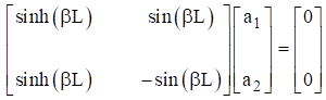
By inspection, equation (8.14) can only be satisfied if and . Set the determinant of the matrix to zero in order to obtain a nontrivial solution. This yields the following transcendental equation. There are multiple roots which satisfy equation. A subscript is thus added.

The equation is satisfied if

The natural frequencies can be found by substituting each root in to equation (8.11).
The solutions to the beam equation for various boundary conditions are derived in Reference [7]. A summary of beam formulas is given in Table 8.1. Note that the free-free beam also has a rigid-body mode with zero frequency.
| Configuration | Fundamental Frequency |
|---|---|
| Cantilever (Fixed-Free) |  |
| Cantilever with end mass |  |
| Pinned-Pinned | 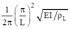 |
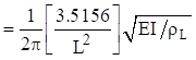
| Free-Free & Fixed-Fixed |  |
| Fixed-Pinned | 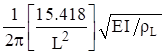 |
The pinned-pinned beam has integer harmonics as follows.

The beam bending frequencies for other configurations have non-integer harmonics. The free-free beam higher modal frequencies are shown in Table 8.2. The free-free formulas also apply to the fixed-fixed beam. The fixed-free beam higher modal frequencies are shown in the following table.
| Mode | Natural Frequency (Hz) |
|---|---|
 |
 |
 |
 |
 |
 |
 |
 |
| Mode | Natural Frequency (Hz) |
|---|---|
|
 |
|
 |
|
 |
|
 |
Again, the mode shapes  and their corresponding mode shapes are found by applying the boundary conditions to the displacement shape in equation (8.9). The participation factors are then

The effective modal mass is


Both the red and blue circles oscillate in the vertical axis in the above figure. The red circle travels at the phase velocity. The blue circle propagates twice as fast at the group velocity and is always at or near the positive or negative peak in the wave packet. The phase speed is the more important of the two speeds for vibroacoustics analyses where the bending waves are excited by the external sound field, or vice versa.
Bending waves are dispersive as a result of the governing fourth-order partial differential equation. The wave speed varies with the angular natural frequency. The phase speed for a given frequency is

The group speed is twice the phase speed.

Demonstrating bending wave propagation in terms of these two speeds is best done with an animation, but the still images in Figure 8.3 may be useful. Furthermore, the phase speed is related to the frequency and bending wavelength by

Natural frequency and modes shapes can also be derived from a beam’s energy terms via the Rayleigh-Ritz or finite element method. The following formulas are given for reference. The total strain or potential energy of a uniform beam is

The total kinetric energy  of a uniform beam is


The area moment of intertia is

The mass per length is

The natural frequency is

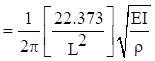
The tallest wind chime was struck separately from the others. The resulting sound was recorded and analyzed. The sound tone represented bending modes. The theoretical value from equation (8.30) agrees closely with the measured frequency 244 Hz. A comparison of the first four bending modes and their respective theoretical values from Table 8.2 is given in Table 8.4. There are two orthogonal planes where transverse vibration occurs. Each mode actually represents a pair of modes. The pair should ideally have the same frequency but may be slightly different due to manufacturing and material imperfections, as well as two holes in each for the connecting cord.
| Mode | Calculated (Hz) | Measured (Hz) | Musical Note |
|---|---|---|---|
| 1 | 238 | 244 | B |
| 2 | 657 | 664 | E |
| 3 | 1288 | 1273 | D# |
| 4 | 2127 | 2050 | C |

The Y-axis represents transverse displacement which has been normalized to have a maximum absolute value of one. The points where each curve crosses the zero baseline are nodal points.

The time history shows some beat frequency effect because each mode is really a pair of orthogonal modes with closely-spaced frequencies.

The highest response is at the fundamental bending mode at 244 Hz. The fourth bending modes at 2050 Hz is barely excited. Note that Fourier transforms are covered in Section 15.
