Free Vibration Model

The mass value is m. The viscous damping coefficient is c. The spring stiffness from Hooke’s law is k. The displacement is x. The velocity is ẋ. The equation of motion is derived using Newton’s law.

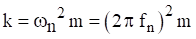
The resulting equation of motion is a second-order, ordinary differential equation, linear, homogenous with constant coefficients. The angular natural frequency in radians/sec is

The natural frequency in cycles/second or Hz is

The natural frequency is the frequency at which the system would oscillate if it were given an initial displacement and then allowed to vibrate freely. The period T is the inverse of the natural frequency.

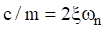
Furthermore, the damping coefficient divided by mass can be represented as

The corresponding amplification factor is

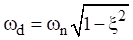
The damped natural frequency is

The free vibration solution to equation (1.3) can found using a Laplace transform and applying the initial displacement and velocity per Reference [2]. The resulting displacement is

The resulting time history is a damped sinusoid, similar to the Pegasus drop transient flight accelerometer data shown later in this document in Figure 10.7.

The conservation of energy method is based on the time derivative of the total energy of an undamped system

Apply this method to the SDOF system in Figure 1.1 to derive the equation of motion.

Dividing through by the velocity term yields the equation of motion for the undamped SDOF system.

The Rayleigh method can be used to determine the fundamental frequency of an undamped system by setting the maximum kinetic energy KE to the maximum potential energy PE.

The kinetic energy for the SDOF system in Figure 1.1 is.

The potential energy for the SDOF system is

Assume a displacement of

The corresponding velocity is

The energy terms become

Substitute the two energy terms into equation (3.1).

Algebraic simplification yields the expected natural frequency

An avionics component is modeled as a solid mass per Figure 1.1. The goal is to mount the component via elastomeric isolator bushings so that the natural frequency is 30 Hz. The isolators will filter out high frequency vibration energy from the base excitation. Calculate the required isolator stiffness using equations (1.4) and (1.5).

The stiffness k in equation (4.2) is the total isolator stiffness. Now assume that the component will be mounted via four isolators in parallel. The individual isolator stiffness would then be 115 lbf/in. The next step would be to determine whether isolators with that stiffness value are commercially available. Otherwise, some adjustment or compromise would be needed.

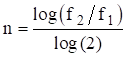
A one octave increase in frequency means that the higher frequency is twice the lower frequency. Conversely, the lower frequency is one-half the higher one. The number of octaves n between any two frequencies f 1 and f 2 is

Note that a piano keyboard has steps of one-twelfth octave counting both the black and white keys.

The octave rule-of-thumb in mechanical vibration analysis states that there should be at least a one octave separation between two frequencies to mitigate dynamic coupling. For example, consider an SDOF system subjected to a harmonic force or base excitation. The system’s natural frequency should be tuned to less than one-half or greater than twice the excitation frequency.

Isolation or low tuning would be the case where the system’s natural frequency was at most one-half the excitation frequency. High tuning occurs when the natural frequency is at least twice the excitation frequency. The system is said to be hard-mounted if the natural frequency significantly greater than the excitation frequency.

As another example, consider two SDOF systems that are to be joined together. The respective natural frequencies should be separated by on octave prior to mounting one with other. The Pegasus launch vehicle in Section 10.6 has a natural frequency of about 10 Hz. The payload’s own natural frequency should be high-tuned to 20 Hz or more to reduce dynamic coupling effects. Note that tuning below 5 Hz is a poor choice due to the possibility of high relative displacement of the payload within the vehicle fairing, as well as possible interference with the autopilot control algorithm stability. Further information about this frequency requirement can be found in the Pegasus Payload User Guide.

Complex variables with real and imaginary components are used extensively in signal analysis and structural dynamics. The imaginary component is expressed as a scale factor applied to

Let C be a complex variable with real component A and imaginary component B.

The variable C is a vector in the complex, Euclidean plane. The magnitude is the norm.

The phase angle is

Euler’s equation is a complex exponential function used for Fourier transforms and for structural modal response.

Complex exponentials can simplify trigonometry, because they are easier to manipulate than their sinusoidal components.